Gridded_composites
Gridded_composites.Rmd
library(compositeR)
library(lipdR)
library(geoChronR)
#> Welcome to geoChronR version 1.1.17!
#>
#> Attaching package: 'geoChronR'
#> The following objects are masked from 'package:lipdR':
#>
#>     createTSid, pullTsVariable
#> The following object is masked from 'package:compositeR':
#>
#>     simulateAutoCorrelatedUncertainty
library(ggplot2)
library(dplyr)
#>
#> Attaching package: 'dplyr'
#> The following objects are masked from 'package:stats':
#>
#>     filter, lag
#> The following objects are masked from 'package:base':
#>
#>     intersect, setdiff, setequal, union
library(tidyr)
library(purrr)
FD <- lipdR::readLipd("http://lipdverse.org/geoChronR-examples/arc2k/Arctic2k.zip")
#> [1] "Loading 19 datasets from /tmp/RtmpWZV55k/lpdDownload..."
#> [1] "reading: Arc-Agassiz.Vinther.2008.lpd"
#> [1] "reading: Arc-Austfonna.Isaksson.2005.lpd"
#> [1] "reading: Arc-CampCentury.Fisher.1969.lpd"
#> [1] "reading: Arc-Crete.Vinther.2010.lpd"
#> [1] "reading: Arc-DevonIceCap.Fisher.1983.lpd"
#> [1] "reading: Arc-Dye.Vinther.2010.lpd"
#> [1] "reading: Arc-GISP2.Grootes.1997.lpd"
#> [1] "reading: Arc-GRIP.Vinther.2010.lpd"
#> [1] "reading: Arc-Hvtrvatn.Larsen.2011.lpd"
#> [1] "reading: Arc-LakeC2.Lamoureux.1996.lpd"
#> [1] "reading: Arc-LakeDonardBaffinIsland.Moore.2001.lpd"
#> [1] "reading: Arc-LakeLehmilampi.Haltia-Hovi.2007.lpd"
#> [1] "reading: Arc-LakeNataujrvi.Ojala.2005.lpd"
#> [1] "reading: Arc-LowerMurrayLake.Cook.2008.lpd"
#> [1] "reading: Arc-NGRIP1.Vinther.2006.lpd"
#> [1] "reading: Arc-NGTB16.Schwager.1998.lpd"
#> [1] "reading: Arc-NGTB18.Schwager.1998.lpd"
#> [1] "reading: Arc-NGTB21.Schwager.1998.lpd"
#> [1] "reading: Arc-Renland.Vinther.2008.lpd"
#>
#>
#> [1] "Successfully loaded 19 datasets, with 0 failure(s)."

FDts <- as.lipdTsTibble(FD)
Create a grid
# Define the boundaries of your grid
min_lat <- 60
max_lat <- 80
min_lon <- -80
max_lon <- 30
# Define the resolution of your grid (in degrees)
resolution <- 10
# Create sequences for latitude and longitude
lats <- seq(min_lat, max_lat, by = resolution)
lons <- seq(min_lon, max_lon, by = resolution)
# Get the lat/lon edges too
latEdges <- seq(min_lat - resolution/2, max_lat + resolution/2, by = resolution)
lonEdges <- seq(min_lon - resolution/2, max_lon + resolution/2, by = resolution)
# Create a grid from these sequences
grid <- expand.grid(lon = lons,lat = lats)
# View the first few rows of the grid
head(grid)
#> lon lat
#> 1 -80 60
#> 2 -70 60
#> 3 -60 60
#> 4 -50 60
#> 5 -40 60
#> 6 -30 60
# Plot the grid on a map
sites <- mapLipd(FD,size = 3) +
geom_hline(yintercept = latEdges, color = "grey80") +
geom_vline(xintercept = lonEdges, color = "grey80") +
geom_point(data = grid, aes(x = lon, y = lat),color = "blue")
sites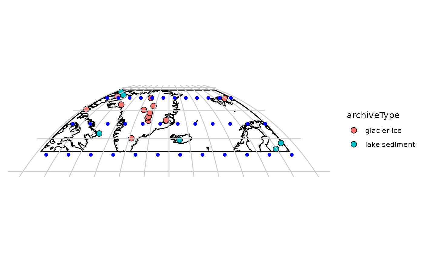 note that the grid df is grid centers, while the edges are the
boundaries of each gridcell
note that the grid df is grid centers, while the edges are the
boundaries of each gridcell
Find the nearest grid point for each dataset
#calculate all the distances between the datasets and each grid cell
allDistances <- map2(FDts$geo_longitude,FDts$geo_latitude,\(x,y) geosphere::distHaversine(c(x,y),as.matrix(grid)))

#find the minimum, and add into the tibble
FDts$cell <- map_dbl(allDistances,which.min)


#make another map to show the number of datasets in each cell
nPerCell <- FDts |>
  select(dataSetName,cell) |>
  distinct() |>
  group_by(cell) |>
  summarize(count = n())


grid$count <- 0 #initialize with zero
grid$count[nPerCell$cell] <- nPerCell$count


baseMap(grid$lon,grid$lat) +
  geom_tile(data = grid,aes(x = lon, y = lat, fill = count),alpha = .5,color = "black") +
  geom_point(data = FDts,aes(x = geo_longitude, y = geo_latitude),colour = "blue",size = 3) +
  scale_fill_viridis_b(right = FALSE)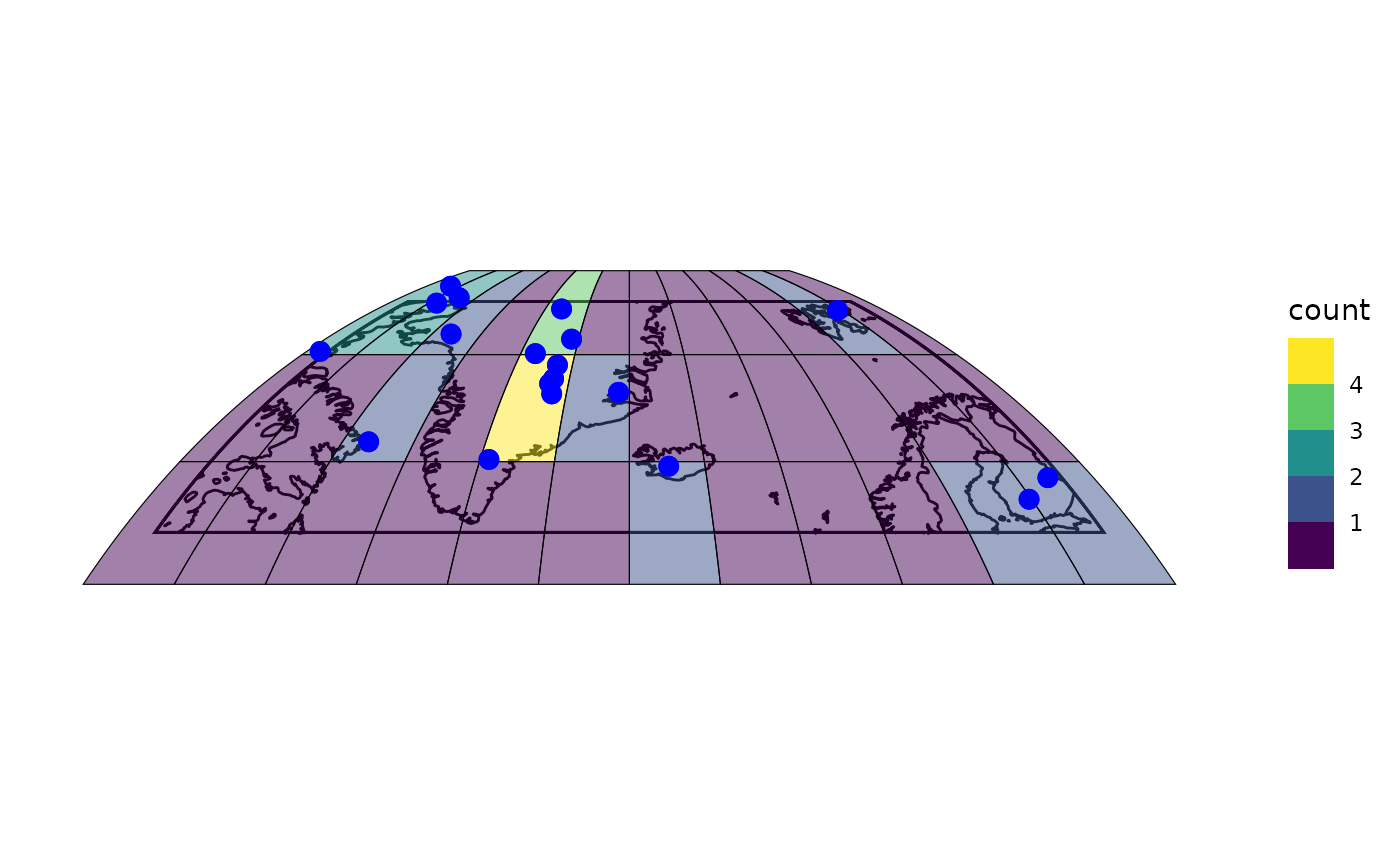
Now, to actually composite these data
Let’s filter the timeseries data down to one value per site.
toComp <- FDts |>
  filter(interpretation1_variable == "T") #select only temperature sensitive timeseries

#now let's use compositeR to create a function that will composite 2 or more datasets within a cell

ourCompositer <- function(cellnum,toComp,binvec){

  thisTS <- filter(toComp,cell == cellnum)

  if(nrow(thisTS) == 0){
    ensOut <- list(ages = rowMeans(cbind(binvec[-1],binvec[-length(binvec)])))

    ensOut$composite <- ensOut$proxyVals <- ensOut$proxyUsed <- matrix(NA, nrow = length(ensOut$ages))

    return(ensOut)

  }else{

  tc <- as.lipdTs(thisTS) |> splitInterpretationByScope()
  ensOut <- compositeEnsembles2(tc,
                                binvec=binvec,
                                ageVar = "year",
                                binFun=sampleEnsembleThenBinTs,
                                stanFun=standardizeOverRandomInterval,
                                normalizeVariance=TRUE,
                                gaussianizeInput = TRUE,
                                nens=100,
                                duration = 200,
                                searchRange=c(1200,2000),
                                minN=5,
                                scale = TRUE #scale composite to mean = 0, sd = 1 after compositing
                              )
  return(ensOut)
  }
}

grid$cell <- seq_along(grid$lat) #number the grid cells
allComps <- map(grid$cell,.f = ourCompositer,toComp = toComp,binvec = seq(0,2000,by = 10))

grid$composites <- allComps

extractMedians <- function(x){
  if(ncol(x$composite) == 1){
    return(tibble(year = x$ages,composite = x$composite))
  }else{
    return(tibble(year = x$ages,composite = apply(x$composite,1,median, na.rm = TRUE)))
  }

}

#pull the medians out of the ensembles
grid$compMedians <- map(allComps,extractMedians)
grid$compMat <- map(allComps,\(x) x$composite)
Now let’s calculate some spatially weighted composites
toCombine <- filter(grid,map_lgl(compMat,\(x) !(all(is.na(x)))))

toCombine$weights <- pracma::cosd(toCombine$lat)
toCombine$weights <- toCombine$weights / sum(toCombine$weights)

toCombine$weightedMat <- map2(toCombine$compMat,toCombine$weights,\(x,y) x*y)

weightedArray <- array(unlist(toCombine$weightedMat),dim = c(nrow(toCombine$weightedMat[[1]]),ncol(toCombine$weightedMat[[1]]),length(toCombine)))

meanArray <- apply(weightedArray,c(1,2),sum,na.rm = TRUE)

plotTimeseriesEnsRibbons(X = toCombine$composites[[1]]$ages,Y = meanArray) +
  scale_x_continuous(breaks = seq(0,2000,by = 100)) +
  labs(x = "Year AD", y = "Area weighted composite",title = "Area Weighted Composite")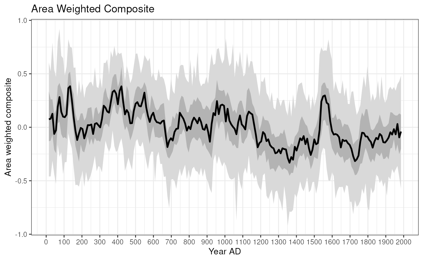
Make some maps of the composites!
#tidy up the data frame for mapping
spatialMedians <- grid |>
  select(-composites) |>
  unnest(compMedians)


#Pick a year to map:
toMap <- filter(spatialMedians,year == 1905)


baseMap(toMap$lon,toMap$lat,f = .2) +
  geom_tile(data = toMap,aes(x = lon, y = lat, fill = composite),alpha = .5,color = "black") +
  scale_fill_distiller(palette = "RdBu",limit = max(abs(toMap$composite),na.rm = TRUE) * c(-1, 1))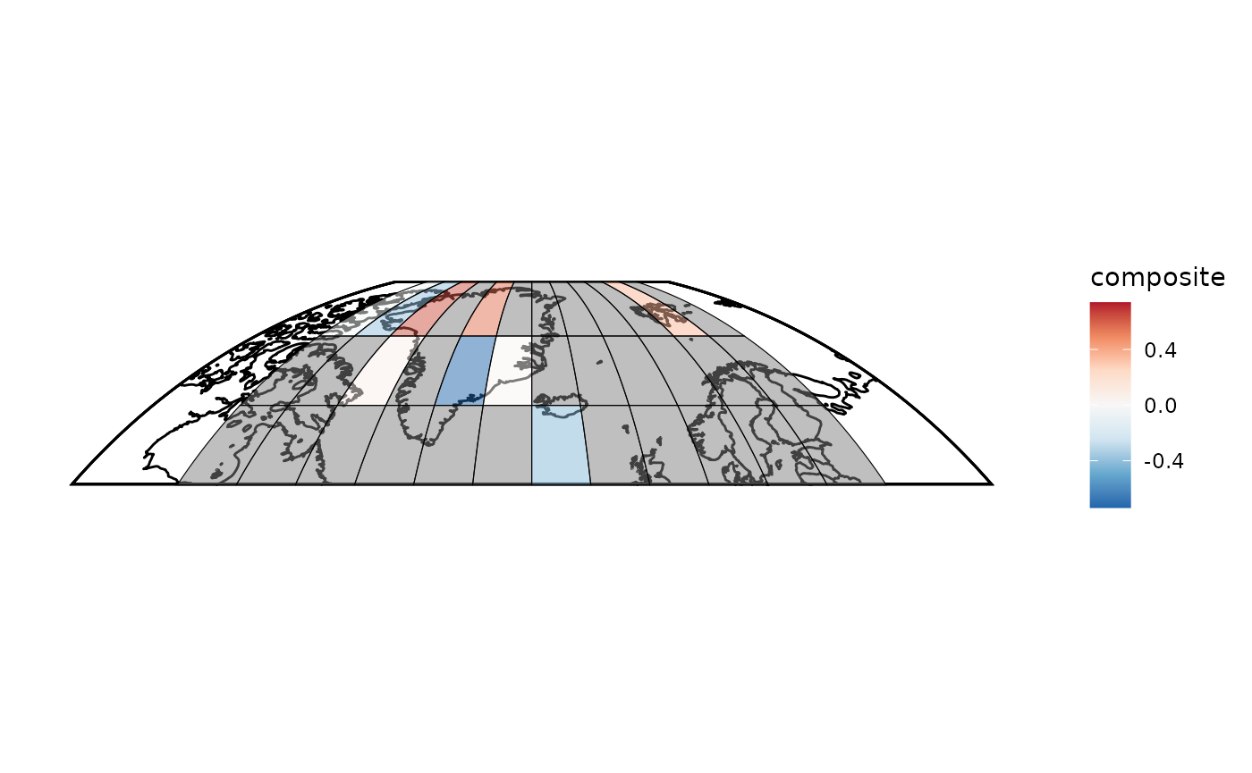
Now can we animate it?
library(gganimate)

anim <- baseMap(spatialMedians$lon, lat = spatialMedians$lat, f = .2) +
  geom_tile(data = spatialMedians,
            aes(x = lon, y = lat, fill = composite),
            alpha = .5,
            color = "black") +
  scale_fill_distiller(palette = "RdBu",
                       limit = max(abs(spatialMedians$composite),
                                   na.rm = TRUE) * c(-1, 1)) +
  labs(title = 'Year: {round(frame_time)}') +
  transition_time(year)

animate(anim)
Gridded composites through time
#some additional code that is useful to save the animation


#create an animation and save it
fps <- 10
animate(anim, fps = fps, duration = length(unique(spatialMedians$year))/fps, width = 800, height = 600,dpi = 150, renderer = gifski_renderer("../preview.gif"))